Highlighting cells • paintr

When you draw a structure to teach with it, you almost always want to point at one part of it, whether this row, that column, or the cells that pass a test. Every paintr painter takes a highlight_area argument for exactly this, and every picture in this article is the same drawing twice, once plain and once with a patch of colour laid over the cells that matter.

A highlight is a logical mask

highlight_area wants a logical structure the same shape as your data, with TRUE wherever a cell should light up and FALSE everywhere else. Nothing more. Here is a small matrix and a mask that turns on its second row by hand.

m <- matrix(1:12, nrow = 3)
mask <- matrix(FALSE, nrow = 3, ncol = 4)
mask[2, ] <- TRUE
mask
#>       [,1]  [,2]  [,3]  [,4]
#> [1,] FALSE FALSE FALSE FALSE
#> [2,]  TRUE  TRUE  TRUE  TRUE
#> [3,] FALSE FALSE FALSE FALSE

paint_matrix(m, highlight_area = mask)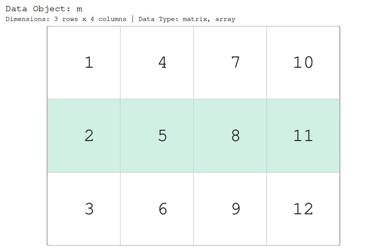

A 3 by 4 grid of the numbers 1 through 12 with its entire second row shaded, so the cells holding 2, 5, 8, and 11 are highlighted while the rest stay plain.

The mask and the data share a shape, so the painter reads them cell for cell. You will rarely build one by hand, though, because paintr gives you a small family of functions that build the mask for you.

The three builders

highlight_data() is the general builder, and three convenience wrappers cover the common cases. Each one returns a mask of the right shape that you hand straight to highlight_area.

highlight_rows() takes a row selection as integer positions, a logical vector, or names when the data has them.

paint_matrix(m, highlight_area = highlight_rows(m, c(1, 3)))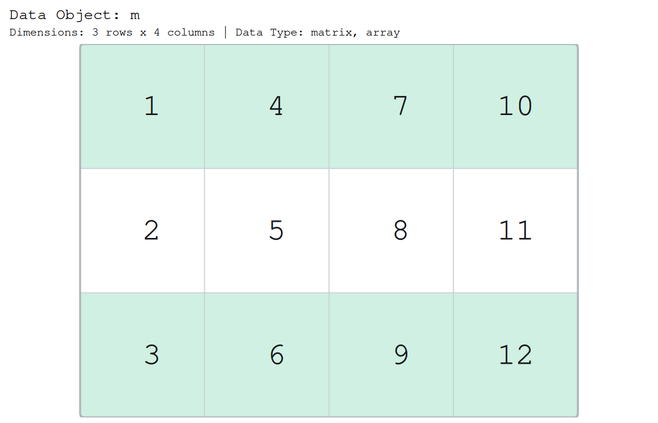

The same 3 by 4 grid of 1 through 12 with its first and third rows shaded, highlighting the cells 1, 4, 7, 10 and 3, 6, 9, 12 while the middle row stays plain.

highlight_columns() takes a column selection the same way.

paint_matrix(m, highlight_area = highlight_columns(m, 2:3))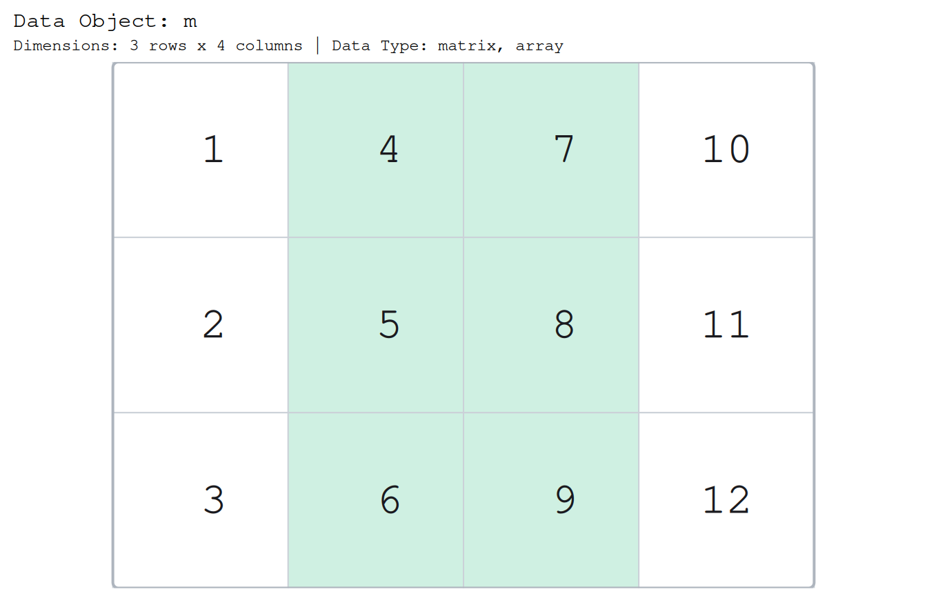

The same 3 by 4 grid with its second and third columns shaded, highlighting the cells 4, 5, 6 and 7, 8, 9.

highlight_locations() reaches individual cells. For a two dimensional structure it takes a two column matrix of row/column pairs, one point per row.

points <- rbind(
  c(1, 1),
  c(2, 3),
  c(3, 4)
)
paint_matrix(m, highlight_area = highlight_locations(m, points))

The same 3 by 4 grid with three individual cells shaded along a diagonal, the values 1, 8, and 12 at positions [1, 1], [2, 3], and [3, 4], while every other cell stays plain.

All three are thin wrappers over highlight_data(), so you can also ask for rows and columns at once and get their union:

paint_matrix(m, highlight_area = highlight_data(m, rows = 1, columns = 4))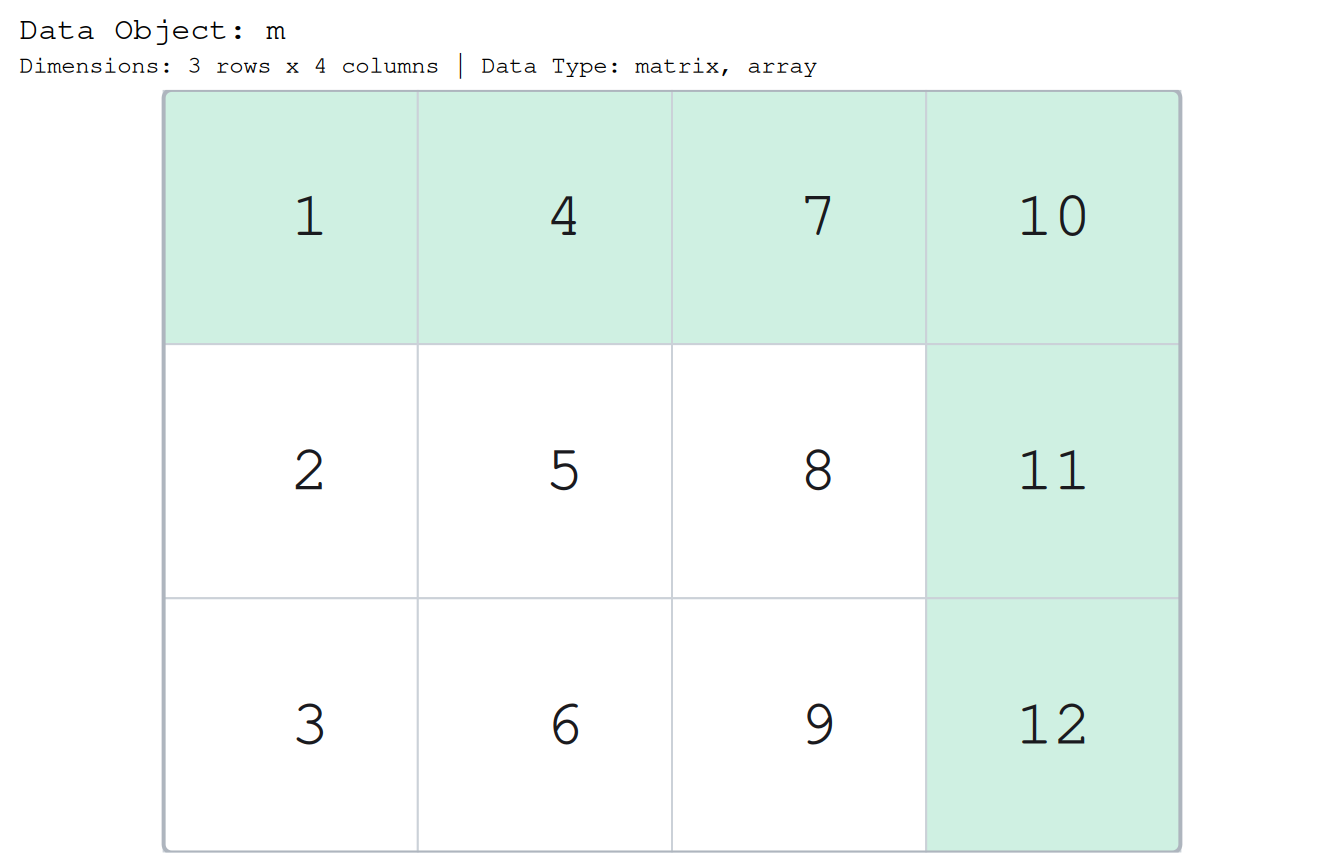

The same 3 by 4 grid with its first row and fourth column both shaded, so the highlighted cells form an L: 1, 4, 7, 10 across the top and 10, 11, 12 down the right edge, meeting at the corner value 10.

A comparison is already a mask

A mask is just a logical the shape of the data, and that is exactly what an R comparison hands back. So you can skip the builders entirely and pass a test:

m > 4
#>       [,1]  [,2] [,3] [,4]
#> [1,] FALSE FALSE TRUE TRUE
#> [2,] FALSE  TRUE TRUE TRUE
#> [3,] FALSE  TRUE TRUE TRUE

paint_matrix(m, highlight_area = m > 4)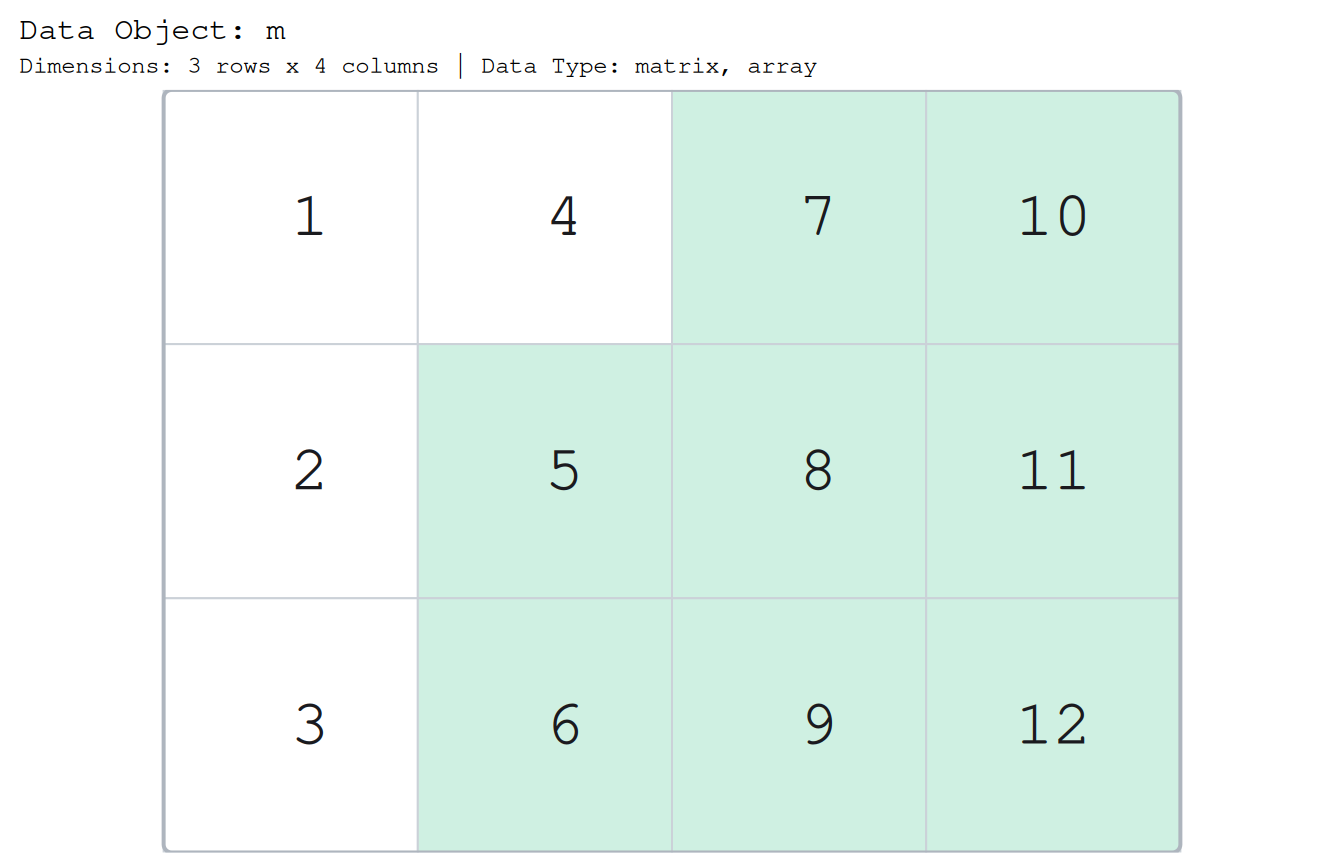

The same 3 by 4 grid with every cell greater than 4 shaded, highlighting the values 5 through 12 while 1, 2, 3, and 4 stay plain; the shaded pattern is exactly the TRUE entries of the comparison m > 4.

The red-and-white grid of m > 4 and the highlighted picture are the same object, the vectorised comparison made visible. which(), is.na(), and friends all produce masks you can drop straight in.

A different colour

The default highlight is a soft "lemonchiffon". Any R colour works through highlight_color:

paint_matrix(m, highlight_area = m > 4, highlight_color = "lightpink")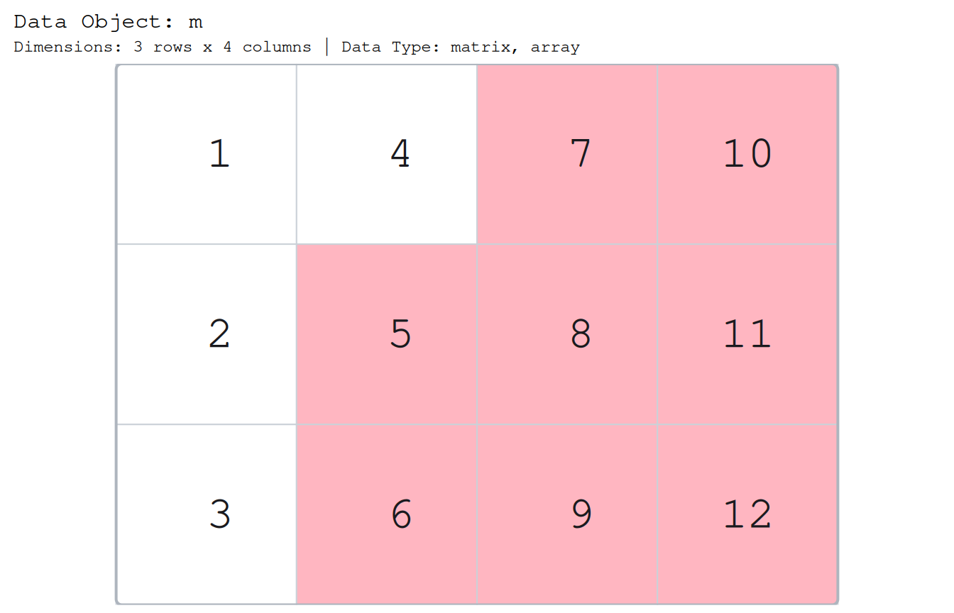

The same grid with cells greater than 4 shaded, this time in light pink rather than the default pale yellow, showing that any R colour can fill the highlighted cells.

Highlighting works on every structure

The invariant is simple. If a painter can draw a structure, highlight_data() can mask it. The builders take the same arguments whatever you point them at, and highlight_columns() in particular will name a column by its name for the structures that have names.

A data frame column, selected by name:

df <- head(iris, 6)
paint_data_frame(df, highlight_area = highlight_columns(df, "Sepal.Width"))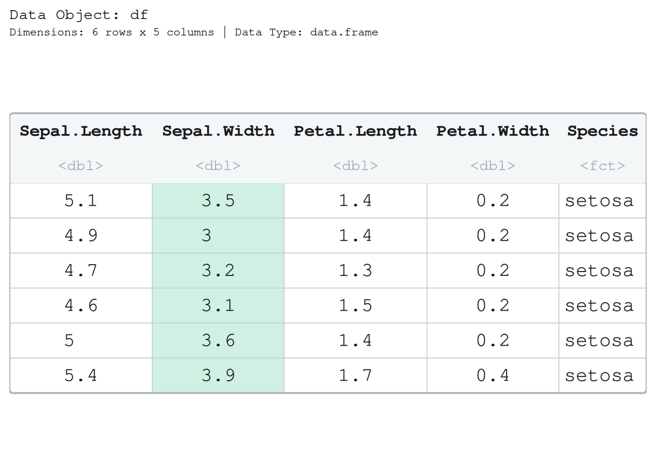

The first six rows of the iris data frame drawn as a table, with the whole Sepal.Width column shaded to pick it out by name from among Sepal.Length, Petal.Length, Petal.Width, and Species.

A list is drawn as its elements side by side, so its elements are its columns. highlight_columns() names one the same way it named a data frame column:

l <- list(counts = c(3, 1, 4, 1), tags = c("a", "b", "c"), ok = c(TRUE, FALSE))
paint_list(l, highlight_area = highlight_columns(l, "tags"))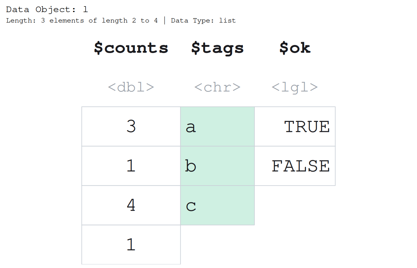

A list drawn as three side-by-side columns headed $counts, $tags, and $ok of decreasing length, so the bottom edge is ragged; the $tags column, holding a, b, c, is shaded to select it by name just as a data frame column would be.

Because a data frame is a list whose elements share a length, and a mask is a mask, the same call reads the same way across the whole family. See vignette("paintr", package = "paintr") for the full tour of the five structures.

Base and ggplot2, the same mask

Highlighting is a property of the drawing, not of the backend, so the mask you build feeds a base picture and a ggplot2 picture without change. The matrices above were base graphics, and here is the identical highlight through gpaint_*:

gpaint_matrix(m, highlight_area = m > 4)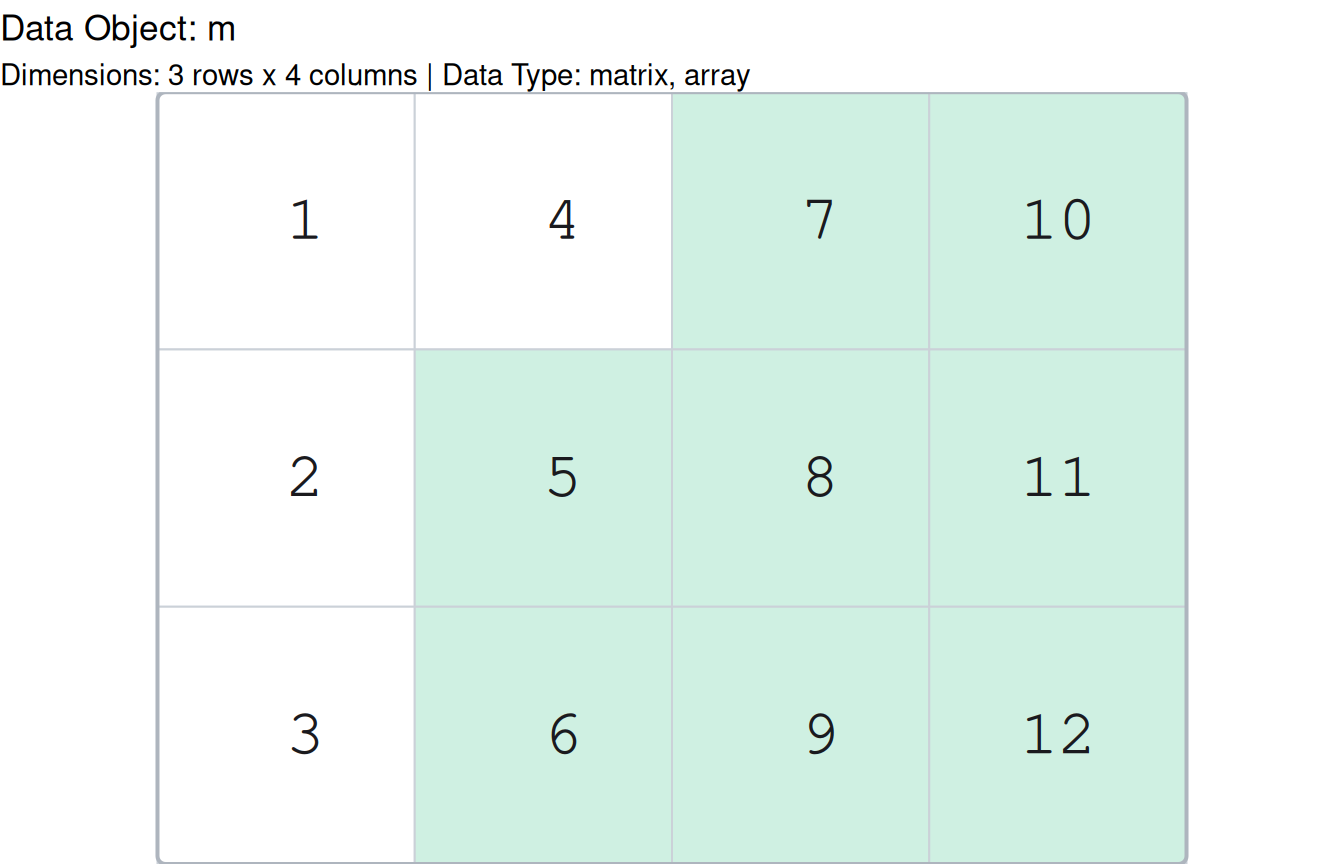

The 3 by 4 grid of 1 through 12 with every cell greater than 4 shaded, drawn through the ggplot2 backend; the highlight is identical to the base-graphics version above, since the mask is a property of the drawing, not the backend.

The paint_* and gpaint_* families take the same highlight_area and highlight_color arguments and mean the same thing by them. For how the two backends differ underneath, see vignette("base-vs-ggplot2", package = "paintr").