emeans fits e-means, the mini-batch alternative to k-means from Meta FAIR’s faiss library, whose authors report a lower loss than Lloyd’s algorithm in about a tenth of the epochs (Bessa et al., 2026; see citation("emeans")). This vignette takes you through a first fit and then the handful of knobs you will rarely need to touch.
The fit is a list holding the centers, each row’s cluster, the sizes and sums of squares familiar from kmeans(), a per-pass history and the recipe that produced it.
summary(fit) prints the recipe with the tail of the history, and since every random draw comes from R’s own generator, set.seed() is all it takes to make a fit reproducible.
Plotting the clusters
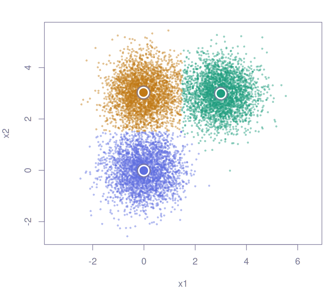
Base graphics are all you need to admire the result: colour each point by its cluster and give each center a ring so it stands out from the crowd.
cols<-c("#1F9E80", "#5F6FE0", "#C27A17")# one colour per clusterplot(x, col =adjustcolor(cols[fit$cluster], alpha.f =0.45), pch =16, cex =0.5, xlab ="x1", ylab ="x2", asp =1)points(fit$centers, pch =21, bg =cols, col ="white", cex =2.4, lwd =2.5)points(fit$centers, pch =1, cex =3.1, lwd =1.5)
Comparison with kmeans()
emeans(x, k) slots into code written for stats::kmeans(x, k), since the result carries the same cluster, centers, size, withinss, tot.withinss, totss and betweenss and answers to predict(); the one difference worth knowing is that iter counts batch updates rather than Lloyd iterations.
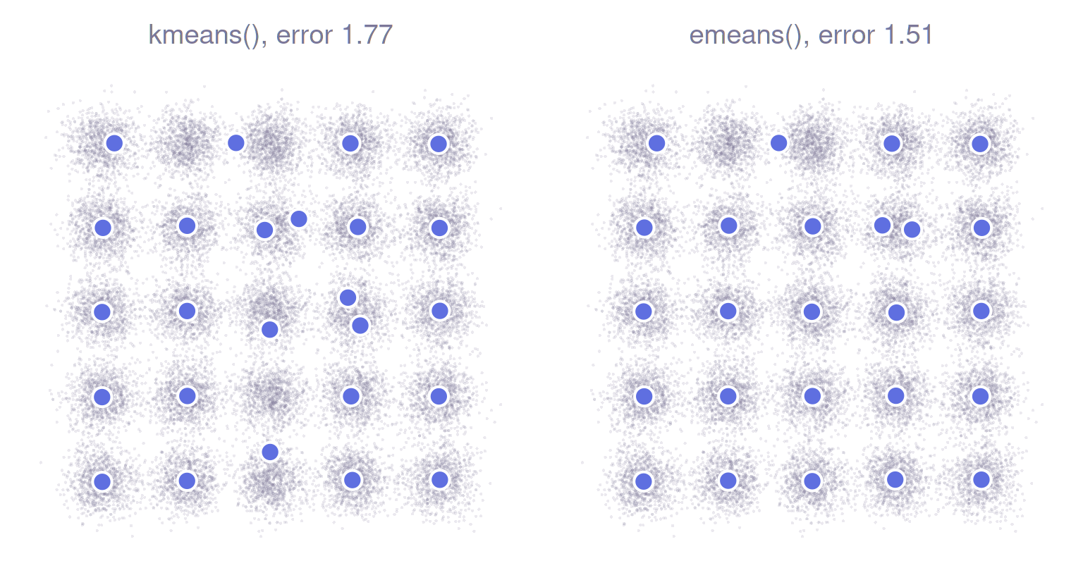
Three well-separated blobs flatter any method, so here is a harder test: 25 blobs on a grid, with both methods starting from the same 25 points and allowed the same number of passes over the data. Each is scored by its error, tot.withinss / nrow(y), the mean squared distance from a point to its nearest center.
Here is where each method stands after six passes:
fits<-list("kmeans()"=lloyd(6), "emeans()"=em6)for(nameinnames(fits)){plot(y, pch =16, cex =0.3, col =adjustcolor("#7C7799", alpha.f =0.15), asp =1, axes =FALSE, xlab ="", ylab ="", main =sprintf("%s, error %.2f", name, fits[[name]]$tot.withinss/nrow(y)))points(fits[[name]]$centers, pch =21, bg =cols[2], col ="white", cex =1.9, lwd =2)}
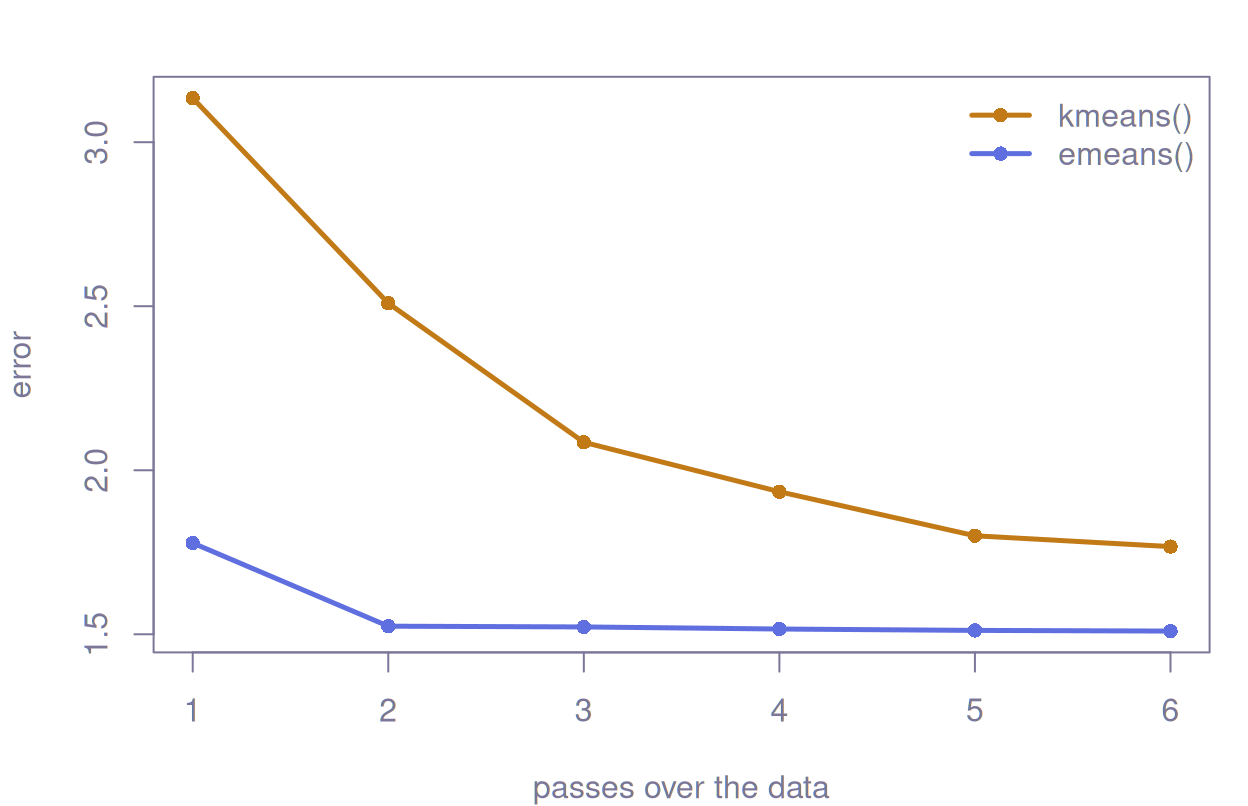
Following the error pass by pass tells the same story. For kmeans() each point on the line is a fresh run allowed one more Lloyd iteration than the last, while e-means logs the error of every pass in fit$history as it goes.
passes<-1:6error<-rbind( kmeans =sapply(passes, function(p)lloyd(p)$tot.withinss/nrow(y)), emeans =em6$history$obj/em6$history$rows)matplot(passes, t(error), type ="o", lty =1, pch =16, lwd =2.5, col =cols[c(3, 2)], xlab ="passes over the data", ylab ="error")legend("topright", c("kmeans()", "emeans()"), col =cols[c(3, 2)], lwd =2.5, pch =16, bty ="n")
Six passes in, Lloyd’s algorithm still has blobs sharing a center while their neighbours go without, whereas e-means does most of its work in the first pass and has settled by the second, although even it leaves one blob with a center to spare.
How the centroids move
Each batch is assigned to its nearest centroids, and every centroid then moves part of the way toward the mean of the batch points it won. How far it moves depends on a weight w that grows with the number of those points and with the step size alpha, while the running count N behind it is an exponential moving average, so old batches fade from memory instead of weighing on the centroid forever.
The step size starts at alpha0 and glides along a cosine to a tenth of that by the last update. During the final pass emeans also keeps each cluster’s exact sums, so every cluster that received points in that pass finishes at their exact mean, a closing flourish that tidies up whatever wobble the moving averages left behind.
The recipe
Left to its own devices, emeans() picks the batch size, the initial step size alpha0 and the revival threshold from the number of rows, k and the dimension, then files the whole recipe away in the fit:
#> List of 4#> $ nepochs : num 5#> $ batch_size: num 64#> $ alpha0 : num 0.295#> $ epoch_rows: num [1:5] 9000 9000 9000 9000 9000
You can override any piece with nepochs, batch_size, alpha0, batch_law or unused_threshold, and nepochs may even be fractional, though a budget so stingy that an epoch would hold no rows is an error.
For the training rows fit$cluster gives the same answer as predict(fit, x), because emeans() finishes with a sweep that labels every row by its nearest final center and adds up the sums of squares on the way. On very large data keep_cluster = FALSE skips that sweep and saves roughly a pass, at the price of the labels and sums of squares. When the fit used max_points_per_centroid, the rows left out of training appear in fit$cluster as NA, though predict() will label them for you.
Spherical mode
With spherical = TRUE, e-means clusters unit vectors by inner product and leaves normalising the data to you.
In this mode predict(type = "distance") returns the inner-product similarity rather than a squared distance, so bigger now means closer.
Odds and ends
threads defaults to getOption("emeans.threads", 2L) and bows to any cap set in the OMP_THREAD_LIMIT environment variable. R for macOS ships without OpenMP, so Mac builds run serially unless you configure the compiler otherwise.
The deliberate differences from the upstream Python implementation are listed under “Differences from upstream” in ?emeans.