Teaching with paintr • paintr

library(paintr)

Four ideas about R’s data structures are worth a whole slide each, and each one is easier to teach as a picture than as a paragraph. This vignette collects them: names versus indices, the sense in which a data frame is a list, the sense in which an array is a stack of matrices, and how to read an accessor straight off a cell. Every picture below is one you can drop into a lecture as is.

Names or indices

A vector can be addressed two ways, and paintr shows you which one you get. Give it a named vector and it draws each name as the accessor you would type, ["NY"] rather than a bare NY, because that is exactly what you write to reach a value.

pop <- c(NY = 8.3, LA = 3.9, Chicago = 2.7)
paint_vector(pop)

A named numeric vector of city populations, 8.3, 3.9, and 2.7, drawn as three cells labelled with their name accessors ["NY"], ["LA"], and ["Chicago"], the expression you type to reach each value.

Take the names away and there is nothing to type but a position, so the picture falls back to [1] [2] [3].

paint_vector(c(3.1, 4.1, 5.9))

An unnamed numeric vector holding 3.1, 4.1, and 5.9 drawn as three cells; with no names to type, the labels fall back to the positional accessors [1], [2], and [3].

That is the whole lesson in two frames: a name is a label you chose, an index is the position that is always there. A matrix works the same way in two dimensions. Give it dimnames and it draws them on both axes.

m <- matrix(c(12, 7, 4, 9, 15, 2), nrow = 2, byrow = TRUE,
            dimnames = list(c("spring", "summer"), c("mon", "tue", "wed")))
paint_matrix(m)

A 2 by 3 matrix with dimnames drawn in the margins as accessors: the rows labelled ["spring", ] and ["summer", ] down the side, the columns [, "mon"], [, "tue"], and [, "wed"] across the top, over the values 12, 7, 4 and 9, 15, 2.

The margins already carry the accessor form: the rows read ["spring", ] and the columns [, "mon"], each a one-sided subscript that names just its own axis. When you want the accessor that reaches a single cell, ask for it: show_indices = "cell" prints the full two-sided subscript under each value. The margins do not go away, so a student sees each axis named on its own and, beneath the number it points at, the combined ["spring", "mon"] that pulls out exactly that value.

paint_matrix(m, show_indices = "cell")

The same 2 by 3 named matrix with each cell now also labelled by its full character subscript, from ["spring", "mon"] in the top-left to ["summer", "wed"] in the bottom-right; the dimname margins remain, so each cell shows both the name on its axis and the accessor that reaches it.

A data frame is a list

This is the strongest single idea in the set, and paintr makes it visible. A data frame is a list whose elements all happen to share a length. Here is a small one.

df <- data.frame(x = c(1.5, 2.5, 3.5), grp = c("a", "b", "c"))
paint_data_frame(df)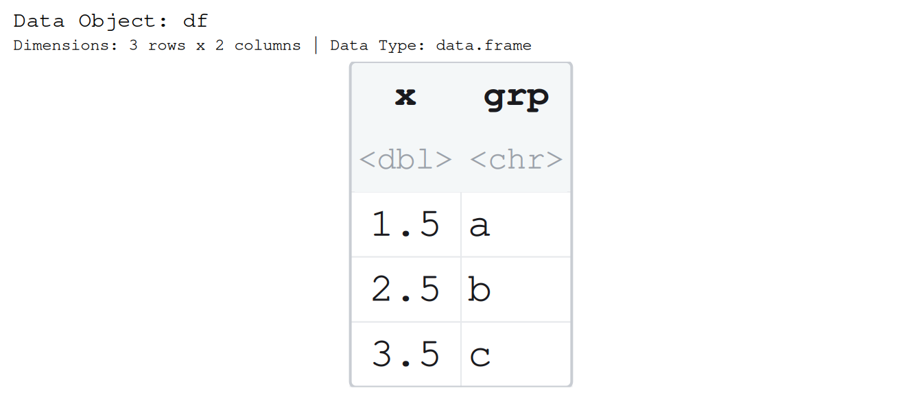

A small data frame drawn as a table with two columns, x holding 1.5, 2.5, 3.5 and grp holding a, b, c, each headed by its bare column name with the column type beneath; the elements share a length, so the table is a clean rectangle.

Now strip the data-frame class away with as.list() and paint the bare list. It is the same picture: the same columns, the same values, the same rectangle.

paint_list(as.list(df))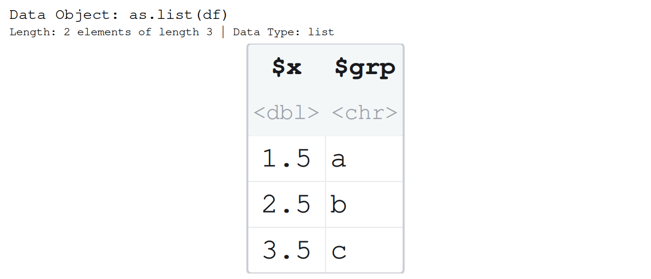

The same data drawn as a bare list after as.list(): two columns headed $x and $grp holding the same values 1.5, 2.5, 3.5 and a, b, c. Because the two elements share a length, the list draws the same clean rectangle a data frame does.

The rectangle is not decoration. The list draws an outline only because its elements share a length – that shared length is exactly the thing that makes a list a data frame. Break it, and watch the rectangle break with it. Here we shorten one column so the elements no longer line up.

broken <- as.list(df)
broken$x <- broken$x[1:2]
paint_list(broken)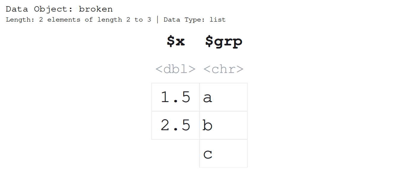

The same list after shortening x to two values, 1.5 and 2.5, while grp keeps three, a, b, c; the elements no longer line up, so the outline is gone and the bottom edge is ragged, the picture of an object that is no longer a data frame.

The outline is gone, because the object is no longer rectangular. data.frame() would have refused to build this. That refusal, and this broken picture, are the same rule seen from two sides: a data frame is a list that stayed a rectangle.

The tight rectangle is a convenience, though, not the truth of the object. A list is a bag of independent vectors that happen, here, to line up. Set gap and the columns move apart to say so – the outline, the mark of a table, falls away.

paint_list(as.list(df), gap = 0.5)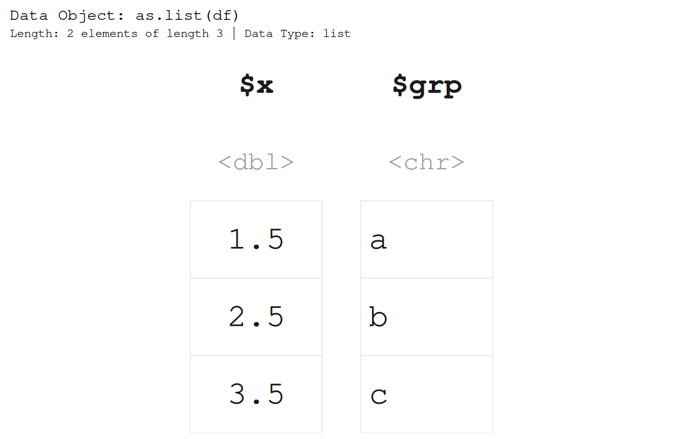

The same equal-length list drawn with gap = 0.5, which pushes the two columns x and grp apart into separate boxed vectors with clear space between them and no enclosing outline; the values are unchanged, but the picture now reads as two independent columns rather than one table.

Same values, same columns, but set side by side rather than fused into a table – which is what a list was all along.

An array is a stack of matrices

A 2-D thing is a matrix; add a dimension and you have a stack of them. paintr draws that stack literally – one block per slice, each block a matrix in its own right, all drawn at one shared font size so the blocks are comparable.

a <- array(1:12, dim = c(2, 3, 2))
paint_array(a)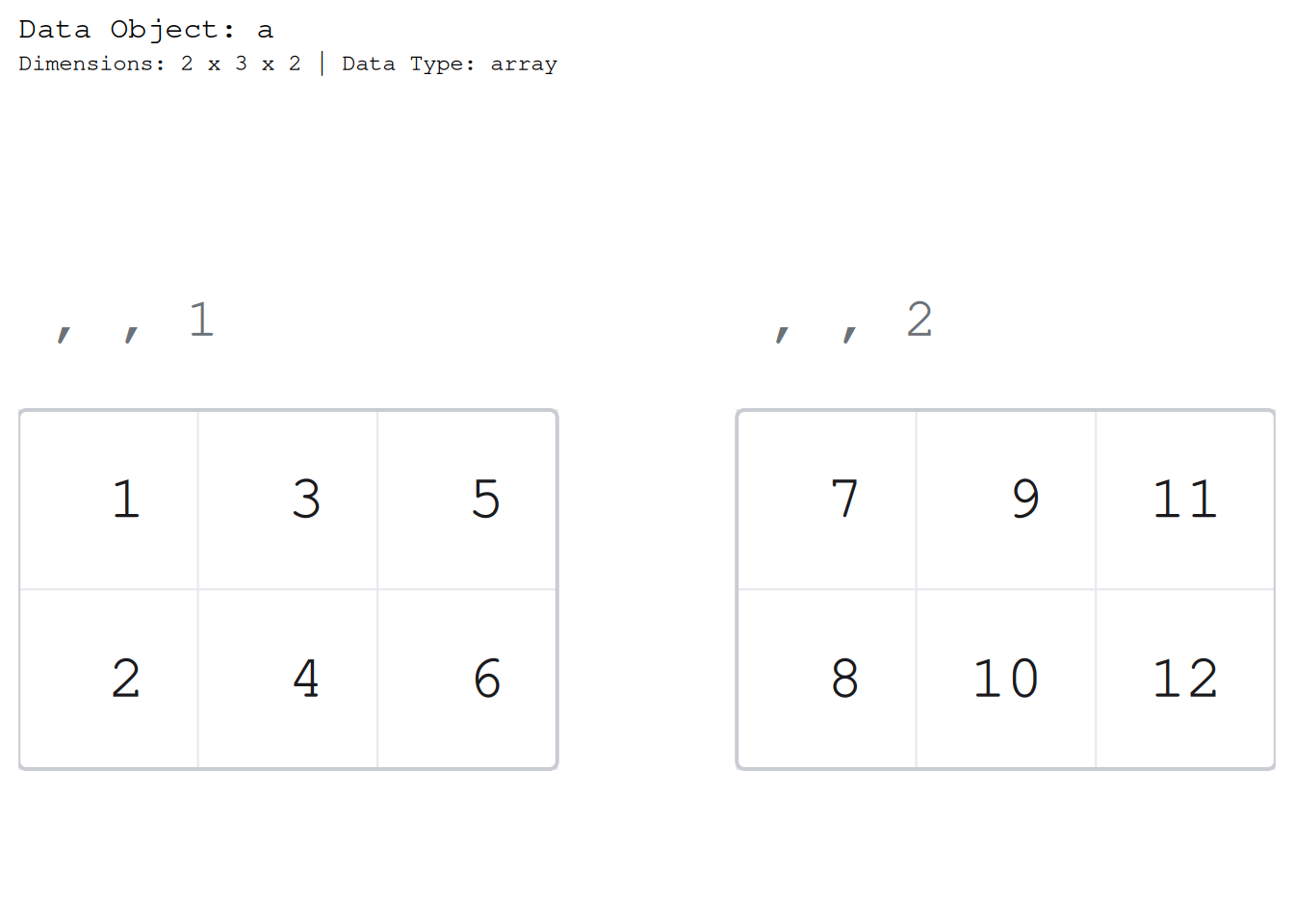

The numbers 1 through 12 drawn as a 2 by 3 by 2 array: two side-by-side blocks, each a 2 by 3 matrix, titled , , 1 and , , 2 in the notation R's own print uses, sharing one font size so the two slices are comparable.

Each block carries the , , k title that R’s own print() uses, so the first block is titled , , 1 and the second , , 2. Read a block on its own and it is an ordinary matrix; the title tells you which slice of the stack you are looking at. That is all a third dimension is: a pile of matrices with a label on each.

Reading an accessor off the picture

The label under a cell is not a caption. It is the exact expression you would type to pull that one value out, printed under the value it returns. This is worth a slide on its own, because it turns the accessor students get wrong most into something they can just read.

Take a list. l[2] is a list, l[[2]] is the vector inside it, and l[[2]][3] is a single value – three expressions that look alike and mean different things. Ask for the indices and paintr writes the right one under each number.

l <- list(a = c(10, 20, 30), b = c(1.5, 2.5))
paint_list(l, show_indices = "cell")

A list of two elements headed $a and $b, holding 10, 20, 30 and 1.5, 2.5, drawn with each cell labelled by its list accessor: double brackets to reach the element then a single bracket to pick the value, so [[2]][2] sits under 2.5 and [[1]][1] under 10.

Under the 2.5 it prints l[[2]][2]: double brackets to reach into the list, single bracket to pick the element. There is no faster way to settle the single-versus-double-bracket confusion than to show the working accessor sitting under the value it produces.

The same trick reads a subscript off an array. Ask a 3-D array for its indices and each cell is labelled with its full three-number subscript.

paint_array(a, show_indices = "cell")

The same 2 by 3 by 2 array with each cell labelled by its full three-number subscript in row, column, slice order; the cell in the second slice, first row, third column reads [1, 3, 2], the exact expression that returns the value it sits under.

The cell in the second slice, first row, third column is labelled a[1, 3, 2] – row, column, slice, in the order R wants them. A student can copy that straight off the picture into the console and get the number it sits under. The picture and the accessor are the same statement.

Where to go next

For the full tour of all five structures and the arguments that shape each picture, see vignette("paintr", package = "paintr"). To turn any of these pictures into a “find the cell” exercise by shading the rows, columns, or values you are asking about, see vignette("highlighting", package = "paintr").